Nanochat
Large Language Models Reinforcement LearningIn the back of my mind, I have known for a while that I have needed to gain a deeper understanding of modern LLM architectures. I have used many of the constituent elements of the architecture for various applications, but I have never implemented an LLM from scratch. One day, all of my machine learning news sources were discussing Andrej Karpathy’s nanochat, an instructive repository that starts at data and ends with a post-trained LLM. The biggest selling point to me was that the entire training curriculum was designed to run locally. The default architecture uses a transformer of depth 20, which trains in 4 hours on an 8xH100 node. I have a more modest 1x3090 node, so I knew that some combination of decreasing my transformer depth and increasing my patience would allow me to start learning to train these models locally.
Preparing the Code
Before I started queuing up long training runs, I identified a few changes to the code that would be necessary. First, let me introduce my first rule of deep learning: Docker is non-negotiable every time, without exception. Let me explain…I have cloned lots of deep learning projects, but this is actually a dangerous exercise if you are not careful. The reason is that implementations often require a specific version of CUDA. CUDA loves to break a functioning linux machine. I can’t tell you how many times I saw experienced, ex-Google engineers lose an entire workday having to reinstall CUDA after accidentally updating to a new minor version. Managing multiple CUDA versions on a single machine sounds like a nice solution, but in my experience it has never worked well. So after playing many hours myself of reinstalling CUDA on Ubuntu, I have created a simple rule that I never allow myself to break: every project gets a Dockerfile. You set up a reasonably recent version of CUDA and pytorch on your machine, and then set tight pins so nothing accidentally gets updated. Then, each project is run via Docker, creating an isolated container that provides the preferred versions of CUDA and other nvidia stack without risking your host machine.
Consequently, the first change I made was to Dockerize the original repo. This came with additional benefits outside of protecting my local machine. When you run through the standard training script, there are many minutes of computation required before pre-training begins. During this time, python packages are downloaded and installed, datasets are downloaded, and a tokenizer is trained using byte pair encoding. Not all of the resulting artifacts are cached by default, which creates optimization opportunities if many models are trained or a single model is trained in multiple campaigns instead of a single run. A properly designed Dockerfile will allow us to cache the resulting artifacts as images, which can easily be reused. I also added a persistent Docker volume to store the downloaded datasets.
Train Time Estimation
With the software considerations out of the way, I next had to think about hardware. The reference machine used to train the default architecture (depth 20 transformer) had access to eight H100 GPUs, while I had a single 3090. Does this present a problem for me? An H100 is a bit faster than a 3090, but there will be some scaling penalty from failing to perfectly scale across 8 GPUs. So one could naively hope that these two factors would cancel out, and consequently I should expect to train 8 times longer, for a slow but palatable 32 hour training run. However, if you know anything about GPU architecture, you will spot many bad assumptions that will tank the quality of this estimate. So let’s think a little more carefully about hardware differences and better predict the time required to train one of these models. Let’s start with comparing the key differences in comparing the datasheets of the cards:
FLOPs
The raw compute is important for training tasks. Comparing the dense FLOPs across these cards, a 3090 achieves about 36 TFLOPs at BF16/FP16, while a single H100 has about 1000 TFLOPs at the same precision. Taken at face value, we would expect training to occur faster by a factor of approximately 28 when comparing a single H100 to a 3090, or a factor of 220 with 8 GPUs. However, the small transformer models will not come anywhere close to saturating the tensor cores due to the small matrix operations. So we would greatly overestimate the training time on a 3090 if we based our estimate on peak FLOPs.
Throughput
If the general matrix multiplication operators will not dominate the training time, where do we spend the training time? For models of this size, training will be limited by memory-dominated kernels, such as attention, layer norm, softmax, embeddings lookups, and optimizer steps. So instead of treating training as FLOPs-bound, we should take the approach that training will be latency-bound and memory-bound. This leaves us comparing a very different set of specifications.
Memory
A single H100 has a memory bandwidth of approximately 3.4 TB/s while a 3090 has 940 GB/s. So the aggregated memory bandwidth will be a factor of 8 higher with the additional GPUs, leading to an aggregate memory bandwidth difference of a factor of 27. The effective memory throughput difference, especially comparing a multi-GPU system to a single card, but we will stick with the factor of 27 for simplicity.
Latency
The next consideration is latency hiding. With multiple GPUs, the latency associated with launching each kernel is naturally amortized across overlapping communication and staggered execution. Additionally, each GPU has more concurrent kernels, and thus more opportunity for overlap in independent streams, further decreasing latency. With a single GPU, every kernel launch lies on the critical path. So when attention, layer norm, MLP, and optimizer kernels are launched, they are forced to serialize. Without any cross-device overlap, there is no slack to hide some of this latency. Without going too deeply in proper modeling, we will estimate a penalty on our single GPU system of 1.4.
Final Estimate
We have estimated that due to the low arithmetic intensity involved with these relatively small models, we will focus on understanding the differences in throughput rather than compute. This led us to adopt a simplistic estimate informed by differences in memory bandwidth and latency. If we simply multiply together these dominant factors, we arrive at a difference of
$27 \times 1.4 \simeq 38$. So we would naively estimate that we would require $38 \times 4$ hours $= 6.3$ days.
Our six day training estimate is certainly not perfect, but it puts us in the ball park of what we should expect for training these models. Moving away from the theory, this number has important ramifications for training these models. I cannot guarantee that my machine will run uninterrupted for almost a week, whether due to an unexpected power outage or crash. Additionally, I may actually want to use my computer at some point in that week, either to work on a different project or to just play Hanabi with friends. Clearly, we need to make software-level changes to capture these hardware-level realities. Specifically, I wanted to ensure that training could be gracefully terminated before completion and easily continued after interruptions. The Dockerfile will help eliminate most of the cold start problem of resuming training, but we need a checkpointing system that keeps track of the model weights in addition to all of the training state information.
For these reasons, I created by own fork of the repo that incorporated these improvements that would be necessary for me to actually run the code and produce a trained model. With these changes in place, I could begin actually dedicate spare GPU cycles towards training my own LLM. I was not ready to commit to a training a full depth-20 model, so I was curious to understand how long it would take to train the smaller models. There are essentially three considerations to estimate the training time of these smaller models:
- The smaller models contain fewer parameters, which will reduce the training time simply from the required computation.
- The smaller models allow for larger batch sizes before I hit out-of-memory issues, which allows for increased throughput.
- The smaller number of parameters results in proportionally smaller training datasets, since the training is Chinchilla-optimal, meaning that the number of training tokens is approximately twenty times the number of free parameters.
I ended up spending most of my time training depth-16 models, since these offered the highest level of performance given my appetite for training time. As a brief aside, I did initialize model training on a depth-20 model simply to check our above napkin math. The training reached 1% right at the 100 minute mark, which would lead to a total training time of about 7 days on my computer. So our rough napkin math held up pretty well despite its simplicity.
Model Training
Pretraining
I was able to train the depth-16 models using a batch size of 8, which almost used up my entire VRAM.

With this batch size, pretraining took about 59 hours to complete on my GPU. Even though these are much smaller models than the default depth-20 models, the need for model checkpointing to allow for resuming training is apparent for my machine.

At the end of this process, I had a neural network with 336M parameters trained on 6.7B tokens. One could think of this pretraining as a procedure condensing 32 billion characters in 336 million parameters. Here is the final benchmark performance of the trained model:
| Task | Accuracy | Centered |
|---|---|---|
| hellaswag_zeroshot | 0.385680 | 0.180907 |
| jeopardy | 0.035427 | 0.035427 |
| bigbench_qa_wikidata | 0.475469 | 0.475469 |
| arc_easy | 0.610269 | 0.480359 |
| arc_challenge | 0.304608 | 0.072810 |
| copa | 0.690000 | 0.380000 |
| commonsense_qa | 0.266175 | 0.082719 |
| piqa | 0.656692 | 0.313384 |
| openbook_qa | 0.350000 | 0.133333 |
| lambada_openai | 0.336697 | 0.336697 |
| hellaswag | 0.387572 | 0.183430 |
| winograd | 0.578755 | 0.157509 |
| winogrande | 0.502762 | 0.005525 |
| bigbench_dyck_languages | 0.095000 | 0.095000 |
| agi_eval_lsat_ar | 0.278261 | 0.097826 |
| bigbench_cs_algorithms | 0.356818 | 0.356818 |
| bigbench_operators | 0.157143 | 0.157143 |
| bigbench_repeat_copy_logic | 0.000000 | 0.000000 |
| squad | 0.132829 | 0.132829 |
| coqa | 0.168608 | 0.168608 |
| boolq | 0.592355 | -0.072751 |
| bigbench_language_identification | 0.252200 | 0.177338 |
| CORE | 0.179563 |
Midtraining + Supervised Fine-Tuning
Unlike pretraining, which attempts to distill a large corpus into a relatively small number of tunable parameters, the goal of midtraining is to reward the model for properly using special tokens reserved for conversation metadata and tools. Next, I performed supervised fine-tuning on the artifact produced by midtraining. Each of these stages has differing memory requirements, so I again tweaked the batch size to maximize throughput without running out of memory.
Evaluation
I could paste in a long list of benchmarks from both the midtraining and supervised fine-tuning stages, but my guess is that no one really cares what these values are. So instead, I will focus on two different evaluations. First, a qualitative evaluation of chatting with final model after SFT. And second, a quantitative evaluation of the performance on GSM8K, which I find a very interesting measure of ability.
Qualitative Evaluation
First, we can ask our trained model a conceptual question to understand how well it can factually answer questions as well correctly infer user intent. Below is a screenshot of chatting with our model after performing SFT to steer it towards imitating a proper chatbot.
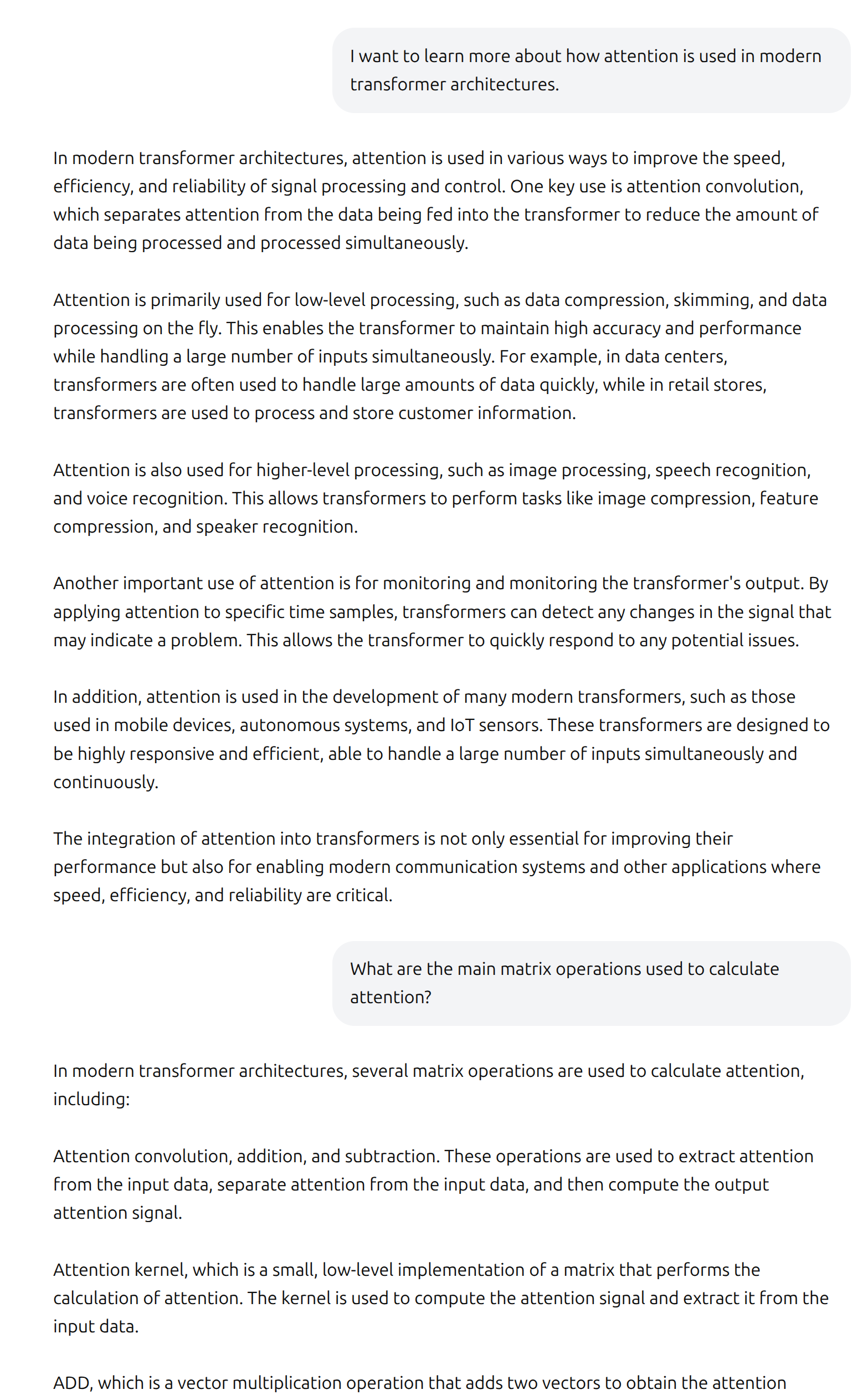
Now, before we are too harsh, it is worth remembering what we are looking at. This is very small language model by modern standards that I was able to train from scratch over a weekend on a very modest one-GPU computer. Truthfully, I did not even know how well it would form complex sentences or use correct grammar. So the ability to meaningfully chat with the model at all is already pretty neat. However, the conversation does admittedly leave something to be desired. The response, while written authoritatively, does not convey any understanding of attention or transformers in the deep learning context.
The follow-up question produced an interesting response. I hoped that the model would mention something about how the key, value, and query matrices are multiplied to form attention scores. After a convoluted detour mentioning “attention convolution” and “attention kernel”, it enumerated a long list of low-level operations, including the “ADD” instruction which was included in the screenshot. The ability to add is certainly required for calculating attention, but clearly this answer misses the intent of the question.
To my surprise, the language model somewhat redeemed itself when asked some simple python questions. I do not expect Anthropic to feel threatened by the coding ability of the model, but it demonstrated a non-trivial ability to write simple functions. The model exhibited several qualities that impressed me. First, it went beyond the straightforward request, providing an example use case with expected output and offering performance-aware improvements. Second, it built upon previous messages to understand the changing requirements of the function.
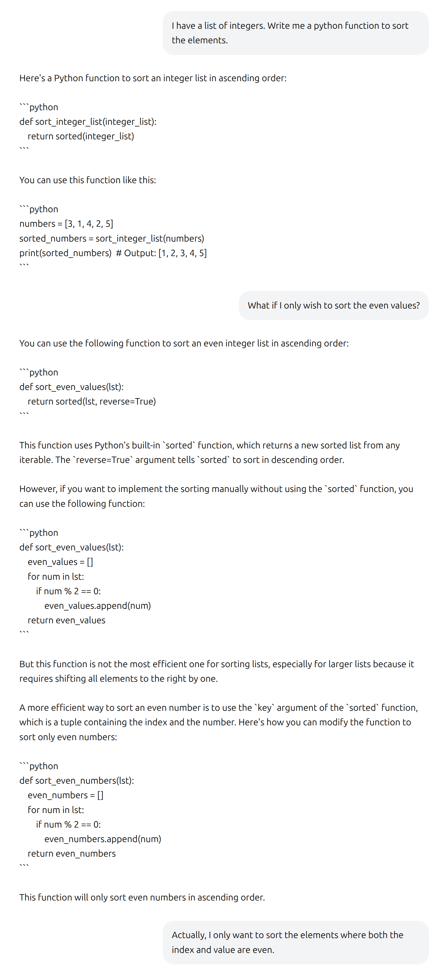
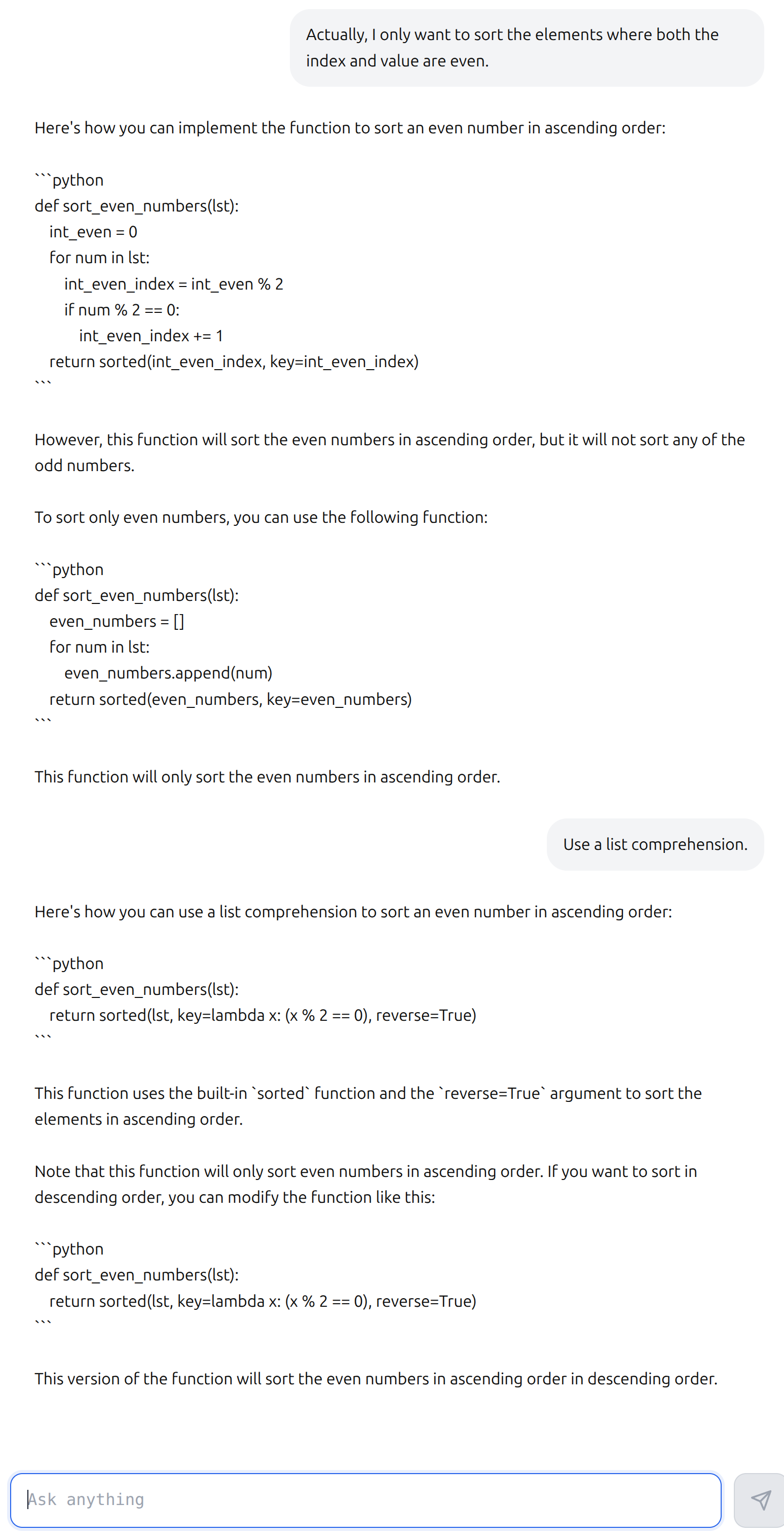
Now, if you look carefully, you can clearly see the flaws in the responses. With the exception of the first response, all of the produced functions contain at least one critical flaw as the task becomes more complicated. The final response, for example, successfully uses a list comprehension, but fails to only sort even numbers or consider the index of elements. Additionally, it provides the same function for both ascending and descending order.
GSM8K Benchmark
Using GSM8K allows us to understand the performance uplift attributable to the different stages of training. Also, we can further optimize performance on this benchmark using reinforcement learning. We observe that the benchmark performance roughly doubles in each stage. The final model, optimized specifically for grade school math problems, may not impress any elementary teachers but outperformed my expectations considering the small parameter count.
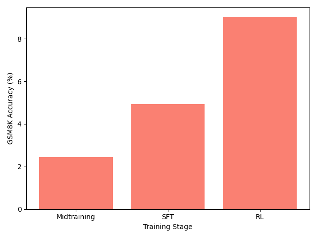
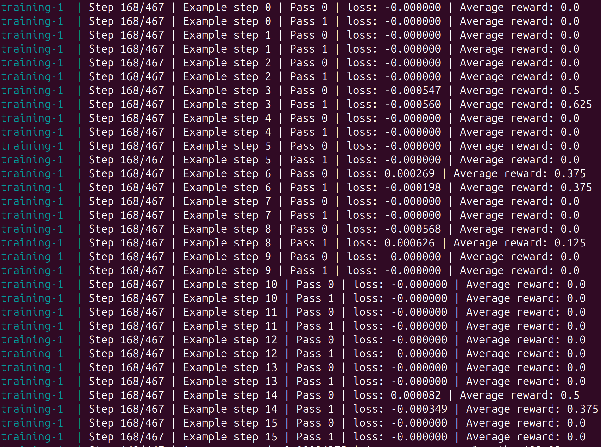
It is worth a slight detour on the limitations of reinforcement learning. The network parameters are only updated with non-zero gradients, which require non-zero rewards to provide a differentiable loss signal. This limits the efficiency of training, particularly when bootstrapping from a model in which rewards are uncommon. For a specific example, the screenshot below illustrates that the network is unable to learn anything from the majority of the steps due to the lack of rewards.
Conclusion
This was a fun and rewarding exercise, and I do feel like I gained a deeper understanding of large language models through getting to train the models from scratch on my own hardware. However, I don’t know if I am satisfied with my level of understanding yet. Andrej Karpathy created a great educational resource with this repo, and I have certainly benefit from all of the work that he put into the code. But I think to truly gain the deep understanding that I want, I actually need to write the model architecture code by hand and be the person that debugs the training loop when the loss does not decrease. I hope to create my own scaled back repo, where I can train a large language model from randomly initialized weights into a model that I can benchmark on different tasks. So I believe this was just the first step in my language model journey.